FDG-PET template construction
To transform PET scans of different rats into a standard space, a template is necessary. Since there is no widely accepted PET template for Sprague-Dawley rats at present, we construct our own template from one existing MRI template [1] using SPM12. The template is ready to download at this website.
PET image preprocessing
The raw images after reconstruction were preprocessed with the constructed template in SPM12. Detailed steps are shown as follows:
- Adjust the voxel size of the images to [9 9 14.4]. In this way, the rat brain can approximately fit the human brain size in order to use the default settings of SPM.
- Adjust all the images into a standard orientation as shown in the example we provided.
- Select on image and align all other images to it using SPM realignment function.
- Align the selected image to the PET template so that the intracranial parts are roughly registered. The transformation parameters are applied to all remaining images so that they are aligned to the template as well.
- After that, co-register all images to the PET template using SPM co-registration function (estimate only).
- Use the parameters from the previous step to reslice the images into the space defined by the ready-to-use image called target.img. The bounding box of the target image is slightly larger than the PET template. The purpose of so-doing is to leave more margin for the next normalization step. The target image can be downloaded from the website.
- (For scans after MCAO only) Replace the injured right hemisphere with the left hemisphere to produce a synthetic and symmetric image. This is because injured areas will contribute much to the cost function during spatial normalization, at the cost of matching accuracy in the healthy areas.
- Normalize the synthetic image spatially to the space defined by the PET template using SPM normalization function (estimate only) and apply the parameters to the original image. For normal (baseline) images taken before MCAO, just normalize the results from step 6 to the PET template. The bounding box is set as [-78 -154 -118; 80 60 6].
- Remove extracranial tissues by a ready-to-use mask image. The mask is a binary image and it is available at our website. People can also make their own mask by segmenting intracranial tissues from the template.
- Smooth all images using a 2mm x 2mm x 4mm isotropic Gaussian kernel.
Extract features using 3D scale invariant feature transform (SIFT) algorithm
After spatial preprocessing, image features were extracted using 3D SIFT method [2]. The Original SIFT is used for 2D images and the detailed algorithm can be found in the original paper by Lowe [3]. Briefly it has four steps:
- Obtain the scale space extrema by calculating the Difference of Gaussian (DoG) and comparing each voxel with its 26 neighbors in a cubic space. The computed extreme voxels are regarded as candidate key points.
- Some candidate key points from last step are removed and others are interpolated for greater accuracy. Thus, the location of scale and space invariant key points are determined.
-
Define the gradient and orientation for each key point. For an image L(x, y), its gradient magnitude m(x, y) and orientation Θ(x; y) are defined as below:
- Obtain a descriptive vector for each key point such that it will be highly distinctive and invariant to location, scaling, translation, rotation and illumination. The descriptor of a key point is constructed from the gradient magnitude and orientation for each sample point in the neighborhood of the key point.
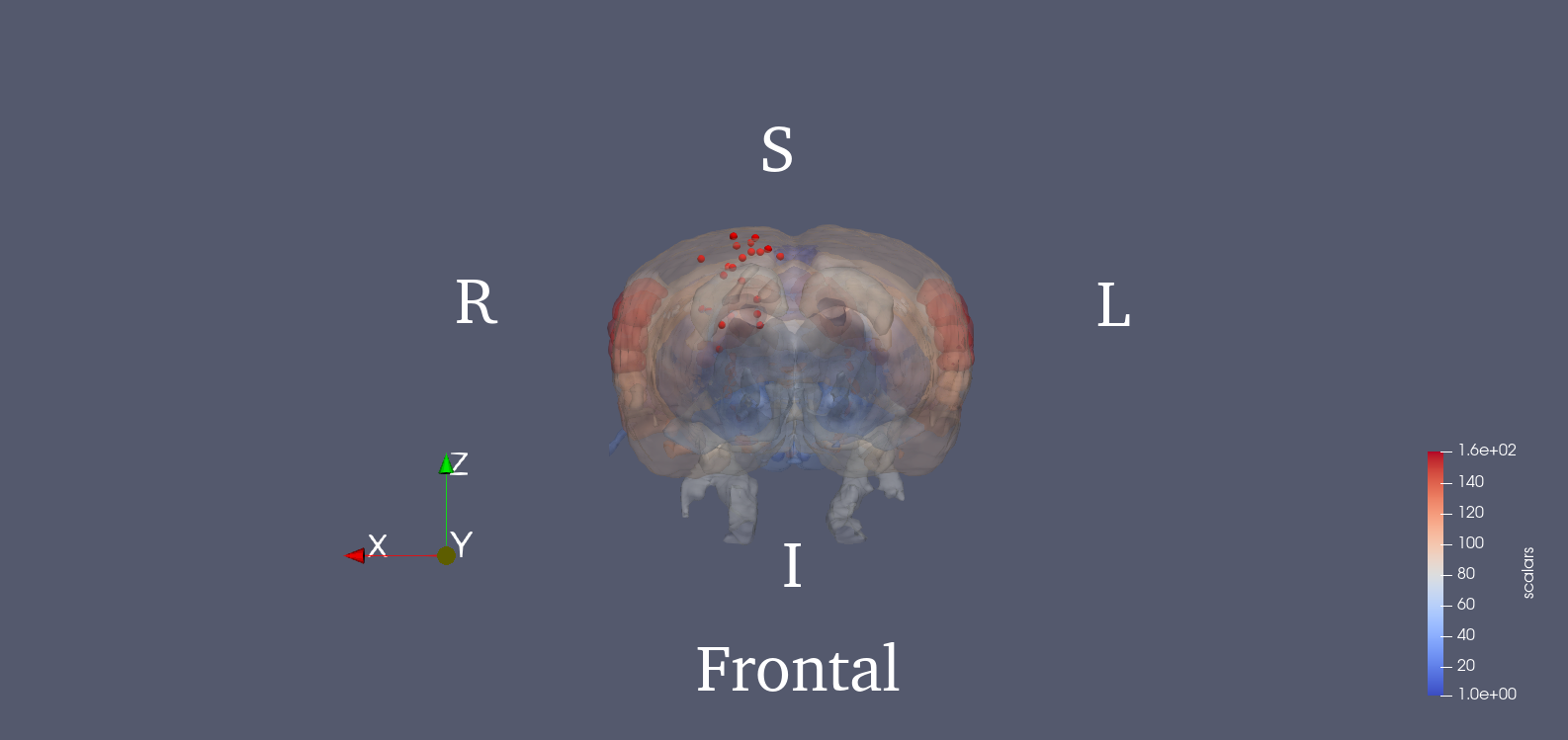
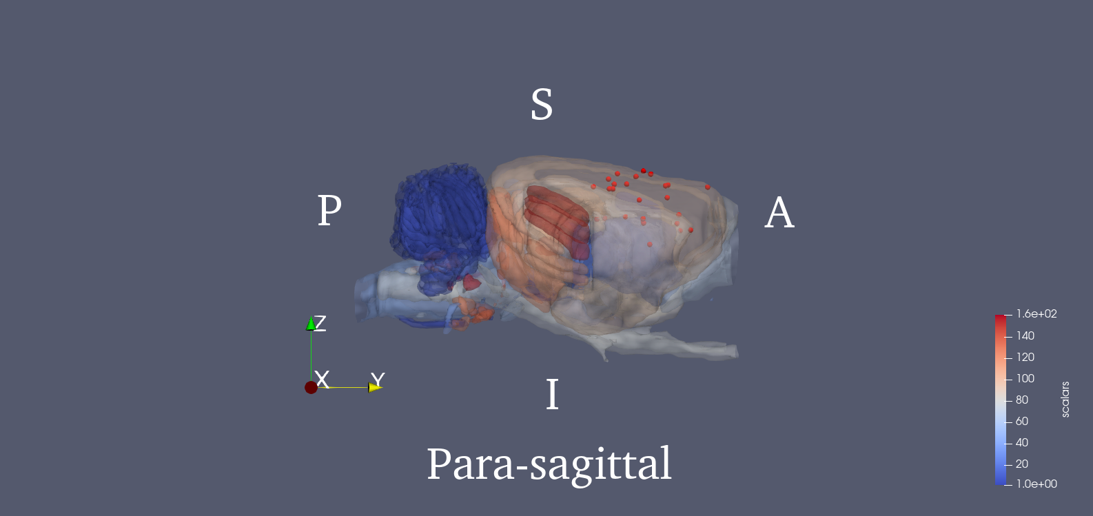
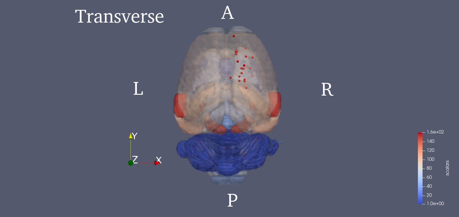
Since PET images were three dimensional, we adopted a 3D SIFT algorithm to extract features. This algorithm extends the notions from 2D SIFT to 3D by using the icosahedral histograms with 12 vertices. In conventional 2D SIFT, the gradient has 8 directions which comes from dividing the planar circle into 8 sectors equally. In the 3D scenario, this algorithm tessellates the sphere into 12 equal tiles. Then the length of a SIFT descriptor will be lifted from 128 to 768. Detailed algorithm of this 3D SIFT can be found in the cited paper [2]. The locations of the 25 key points are provided in the .mat file. We also show the 3D rendered figure for visualization using ParaView [4]. The 25 key points were chosen from potentially affected brain regions during stroke, and the SIFT descriptor of each one is calculated. Brain region delineation is based on the Waxholm atlas (3rd version) [5]. Then, the 25 descriptors will be concatenated into a single vector, which becomes the image feature.
Links
Statistical Parametric Mapping3D SIFT
Waxholm rat atlas
Reference
[1] Schweinhardt, P., Fransson, P., Olson, L., Spenger, C., & Andersson, J. L. (2003). A template for spatial normalisation of MR images of the rat brain. Journal of neuroscience methods, 129(2), 105-113.
[2] Rister, B., Reiter, D., Zhang, H., Volz, D., Horowitz, M., Gabr, R. E., & Cavallaro, J. R. (2015, September). Scale-and orientation-invariant keypoints in higher-dimensional data. In 2015 IEEE International Conference on Image Processing (ICIP) (pp. 3490-3494). IEEE.
[3] Lowe, D. G. (2004). Distinctive image features from scale-invariant keypoints. International journal of computer vision, 60(2), 91-110.
[4] Ahrens, J., Geveci, B., & Law, C. (2005). Paraview: An end-user tool for large data visualization. The visualization handbook, 717.
[5] Papp, E. A., Leergaard, T. B., Calabrese, E., Johnson, G. A., & Bjaalie, J. G. (2014). Waxholm Space atlas of the Sprague Dawley rat brain. Neuroimage, 97, 374-386.